mlkem768-encaps/openssl
|
|
Additional Statistics:
| Lower bound | Estimate | Upper bound | |
|---|---|---|---|
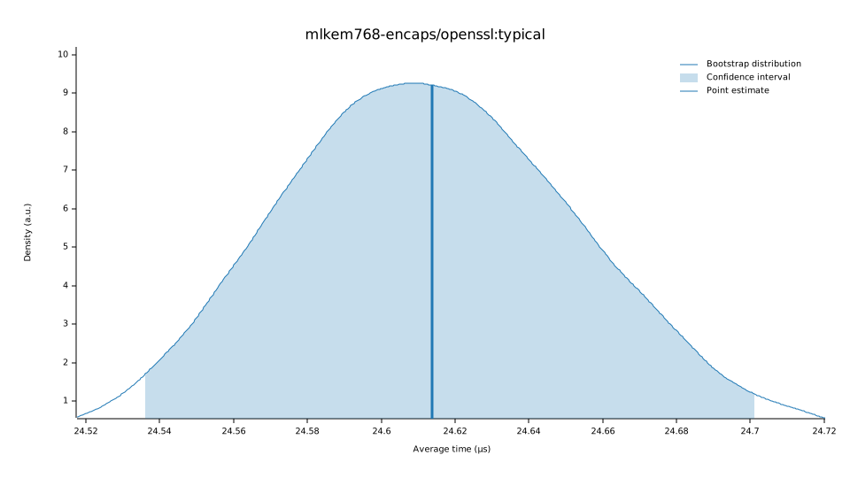
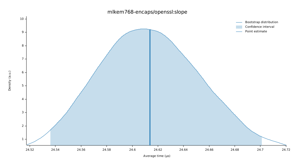
| Slope | 24.536 µs | 24.614 µs | 24.702 µs |
| Throughput | 40.483 Kelem/s | 40.628 Kelem/s | 40.757 Kelem/s |
| R² | 0.9738013 | 0.9751665 | 0.9734304 |
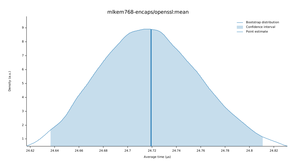
| Mean | 24.637 µs | 24.719 µs | 24.812 µs |
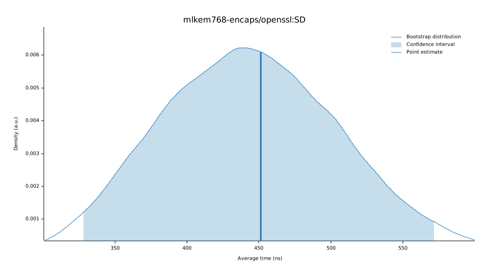
| Std. Dev. | 327.96 ns | 451.23 ns | 572.50 ns |
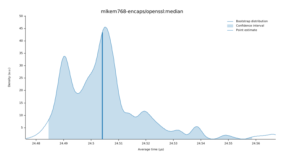
| Median | 24.484 µs | 24.504 µs | 24.559 µs |
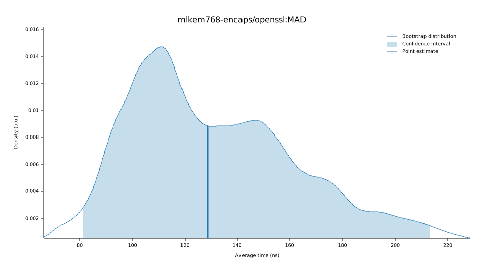
| MAD | 80.976 ns | 128.69 ns | 213.58 ns |
Understanding this report:
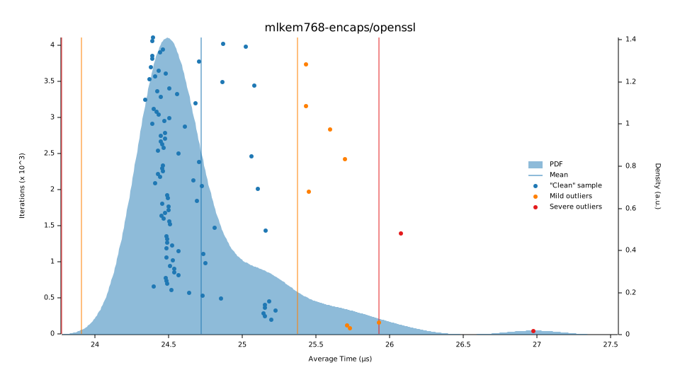
The plot on the left displays the average time per iteration for this benchmark. The shaded region shows the estimated probability of an iteration taking a certain amount of time, while the line shows the mean. Click on the plot for a larger view showing the outliers.
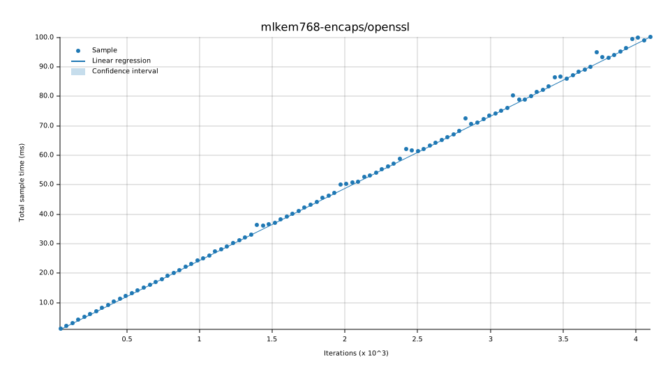
The plot on the right shows the linear regression calculated from the measurements. Each point represents a sample, though here it shows the total time for the sample rather than time per iteration. The line is the line of best fit for these measurements.
See the documentation for more details on the additional statistics.